Lenapy for spherical harmonics and gravity data
Lenapy includes functions to read and process spherical harmonics and gravity data.
These function are accessible to be applied to a dataset using xarray accessor. With a xr.Dataset instance ds, one can call the function to be applied onto ds with ds.lnharmo.func().
The corresponding functions are located in the package lenapy.utils (for lnharmo it corresponds to function mainly from lenapy.utils.harmo and lenapy.utils.gravity).
Imports
Lenapy is an overlayer of xarray. For using lenapy fonctionnalities you need to import both xarray and lenapy.
[32]:
import xarray as xr
import lenapy

import os
import numpy as np

# for plotting:
import matplotlib.pyplot as plt
import cartopy.crs as ccrs
Reading
Reader implemented in lenapy are an overlayer for the xr.open_dataset() function of xarray. To use this reader, you need to modify the argument engine= with ‘lenapyGfc’ or ‘lenapyGraceL2’.
The data are loaded into a dataset with ‘clm’ and ‘slm’ variables. If errors information are available they are load into ‘eclm’ and ‘eslm’ variables.
Metadata informations are saved into attributs accesible with ds.attrs
ascii file with .gfc format reading
File that follow the .gfc format can be read with lenapy (https://icgem.gfz-potsdam.de/docs/ICGEM-Format-2023.pdf) using engine=’lenapyGfc’.
If the model name (in the header of the .gfc file) does not contain date information, use no_date=True.
The reader ‘lenapyGfc’ can be given date_regex and date_format arguments to specify the exact date information. See the function documentation for more details.
You can download the corresponding files on the ICGEM website.
gfct temporal files
If your .gfc file contains temporal informations in the format icgem1.0 or icgem2.0, it can be read with lenapy too.
You then need to use the function lenapy.utils.gravity.gfct_field_estimation() to estimate the gravity field at certain dates.
[33]:
# April 2002 .gfc from GRAZ center
file = '../../data/GSM-2_2002213-2002243_GRAC_COSTG_BF01_0100.gfc'

ds = xr.open_dataset(file, engine='lenapyGfc', no_date=False)
ds
[33]:
<xarray.Dataset> Size: 266kB
Dimensions:     (l: 91, m: 91, time: 1)
Coordinates:
  * l           (l) int64 728B 0 1 2 3 4 5 6 7 8 ... 82 83 84 85 86 87 88 89 90
  * m           (m) int64 728B 0 1 2 3 4 5 6 7 8 ... 82 83 84 85 86 87 88 89 90
  * time        (time) datetime64[ns] 8B 2002-08-16T12:00:00
Data variables:
    clm         (l, m, time) float64 66kB ...
    slm         (l, m, time) float64 66kB ...
    eclm        (l, m, time) float64 66kB ...
    eslm        (l, m, time) float64 66kB ...
    begin_time  (time) datetime64[ns] 8B ...
    end_time    (time) datetime64[ns] 8B ...
    exact_time  (time) datetime64[ns] 8B ...
Attributes:
    product_name:            GSM-2_2002213-2002243_GRAC_COSTG_BF01_0100
    earth_gravity_constant:  398600441500000.0
    radius:                  6378136.3
    norm:                    4pi
    tide_system:             tide_free
    max_degree:              90
    errors:                  empirical
modelname: GSM-2_2002213-2002243_GRAC_COSTG_BF01_0100The dataset is composed of three dimensions : l for the degree dimension, m for the order dimension and time for the temporal dimension.
It contains clm and slm variables that are 3D array corresponding to Stokes coefficients. If the corresponding informations are available in the original file, the formal errors of Stokes coefficients are loaded in variables eclm and eslm and temporal informations corresponding of the first/last date of the data used to create the file as well as the exact time of the date between first and last date are stored.
The attributes of the dataset (ds.attrs) contain metadata information related to the Stokes coefficients
Multifiles
We can also use xr.open_mfdatasets() to open multiple files.
For example you can load a list of the files in a directory with
files = os.listdir(folder_path)
ds = xr.open_mfdataset(files, engine=’lenapyGfc’, combine_attrs=”drop_conflicts”)
ascii file with Level 2 GRACE format
File from GRACE Level-2 SDS centers (CSR, GFZ, JPL) and from CNES can be read with engine=’lenapyGraceL2’.
You can download CNES files here or CSR/GFZ/JPL files here.
The reading works for compressed files. For example : > file_csr = os.path.join(folder_path, ‘GSM-2_2002213-2002243_GRAC_UTCSR_BB01_0600.gz’ > > ds_csr = xr.open_dataset(file_csr, engine=’lenapyGraceL2’)
Apply L2 -> L2B coefficient corrections
For the following demonstration, we use COST-G products (GRACE RL01 + GRACE-FO operational RL02) between 2002 and December 2022.
[50]:
# Dataset with COST-G months of GRACE and GRACE-FO
ds_path = '../../data/COSTG_n12_2002_2022.nc'

ds = xr.open_dataset(ds_path)
Apply simple spatial filtering
GRACE products need to be filtered to remove north-south striping. It can be done with a gaussian filter in lenapy.
[51]:
from lenapy.utils.gravity import gauss_weights

# radius in meters
ds_gauss_weights = gauss_weights(radius=300000, lmax=12)

ds_filtered = ds.lnharmo * ds_gauss_weights
Read TN14
Both TN14 and TN13 dataset can be download here : https://podaac.jpl.nasa.gov/gravity/grace-documentation#TechnicalNotes
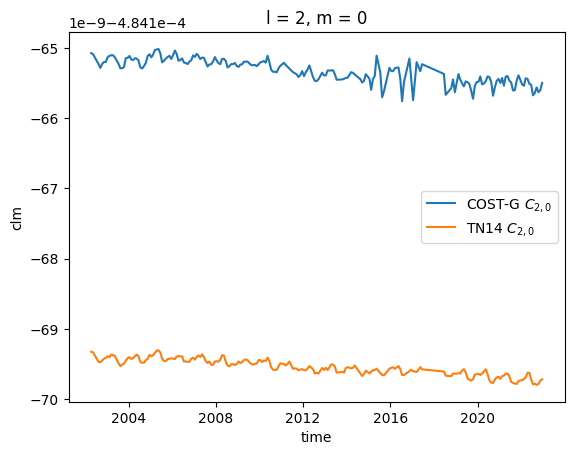
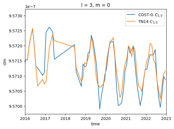
\(C_{2,0}\) coefficient has a large uncertainty for GRACE products compared to other determination with SLR satellites. It is the same for \(C_{3,0}\) coefficient after August 2016 and the accelerometer failure of one GRACE and GRACE-FO satellite.
To improve the quality of GRACE products, supplementary dataset, TN14, that can be used to corrected these coefficients is delivered by the processing centers.
The function read the time-series with or without the mean value using the argument rmmean= (False by default).
[52]:
from lenapy.readers.gravi_reader import read_tn14, read_tn13

ds_C20_C30 = read_tn14('../../data/TN-14_C30_C20_GSFC_SLR.txt', rmmean=False)
To be really precise, you need to change the Earth radius associated to the coefficients used for the correction so that it correspond to the constant associated the the GRACE product used (COST-G here) and then you can replace the coefficients in the product.
The function change_reference() read the ‘radius’ and ‘earth_gravity_constant’ initial and final variables from the dataset.attrs or they can be given with optionnal attributes of the function.
Note that the modification for coefficient :math:`C_{2,0}` and :math:`C_{3,0}` is negligeable
[53]:
from lenapy.utils.gravity import change_reference

ds_C20_C30 = change_reference(ds_C20_C30, new_radius=ds.attrs['radius'], new_earth_gravity_constant=ds.attrs['earth_gravity_constant'])

ds.clm.sel(l=2, m=0).plot(label='COST-G $C_{2,0}$')
# Correct C20
ds.clm.loc[{'l':2, 'm':0}] = ds_C20_C30.clm.sel(l=2, m=0, time=ds.time)
ds.clm.sel(l=2, m=0).plot(label='TN14 $C_{2,0}$')
plt.legend()

plt.figure()
ds.clm.sel(l=3, m=0).plot(label='COST-G $C_{3,0}$')
# Correct C30 after July 2016 for GRACE and GRACE-FO (start on August 2016)
ds.clm.loc[{'l':3, 'm':0, 'time':slice('2016-08-01', None)}] = ds_C20_C30.clm.sel(l=3, m=0, time=slice('2016-08-01', str(ds.time.values[-1])[:10]))
ds.clm.sel(l=3, m=0).plot(label='TN14 $C_{3,0}$')
plt.xlim(np.datetime64('2016-01-01'), np.datetime64('2023-01-01'))
plt.legend()
[53]:
<matplotlib.legend.Legend at 0x71d50c0ffe10>
Read TN13
GRACE products does not contain degree 1 coefficients and are then referenced with an origin corresponding to the center of mass of the Earth. To add degree 1 coefficient, processing centers are delevering TN13, degree 1 time-series product. Each SDS centers has is own TN13 file that is generated with center products using Sun et al. 2016 and Swenson et al. 2008.
To read and apply the correction
ds_deg1 = lenapy.readers.gravi_reader.read_tn13(‘TN-13_GEOC_CSR_RL06.2.txt’)
ds.clm.loc[{‘l’:1, ‘m’:0}] = ds_deg1.clm.sel(l=1, m=0, time=ds.time)
ds.clm.loc[{‘l’:1, ‘m’:1}] = ds_deg1.clm.sel(l=1, m=1, time=ds.time)
ds.slm.loc[{‘l’:1, ‘m’:1}] = ds_deg1.slm.sel(l=1, m=1, time=ds.time)
Projecting spherical harmonics into spatial grid
Details of the projection
\(C_{l,m}\) and \(S_{l,m}\) coefficients can be projected on a grid with an associated radius \(R\) using the formula:
\(\eta(\lambda, \theta) = \sum_{l=0}^{l_{max}} \zeta_l \sum_{m=0}^{l} \lbrack C_{l,m}\cos(m\lambda) + S_{l,m}\sin(m\lambda)\rbrack P_{l,m}(\cos \theta)\)
\(\lambda\) is the longitude, \(\theta\) is the colatitude, \(P_{l,m}\) are normalized Legendre polynomials.
By default, the \(R\) correspond to ds.attrs[‘radius’] but it can be changed with lenapy.utils.gravi.change_reference().
EWH (default unit)
To project onto Equivalent Water Height unit, in the above formula:
\(\zeta_l = \frac{R\rho_{earth}}{3\rho_{water}}~\frac{2l+1}{1+k_l}\)
With \(\rho_{earth}\) the mean earth density, \(\rho_{water}\) the water density, \(k_l\) the potential loading love numbers and \(R\) the Earth mean equatorial radius.
The using R correspond to ds.attrs[‘radius’].
Other units
You can also transform Stokes coefficients into different units with appropriate \(\zeta_l\).
Here is a list of the units :
‘mewh’ for meters of EWH
‘geoid’ for millimeters geoid height
‘microGal’ for microGal gravity perturbation
‘potential’ for meters2.seconds-2
‘pascal’ for equivalent surface pressure
‘mvcu’ for meters viscoelastic crustal uplift
‘mecu’ for meters elastic crustal deformation
Function for the conversion
The conversion can be used as a method onto the dataset with an accessor: ds.lnharmo.to_grid()
This writing is equivalent to sh_to_grid(ds) (located in lenapy.utils.harmo) so to see the argument that might be used look at the documentation of this function.
You can change the degree \(l\) and order \(m\) that are used for the conversion, change the longitude and the latitude of projection and use an ellispoidal Earth. Using kwargs, you can also pass parameters to l_factor_conv** to change the used constants in the unit conversion.
[54]:
from lenapy.utils.harmo import sh_to_grid

# by default, unit='mewh' for meters of equivalent water height
grid = ds.lnharmo.to_grid()

# other unit can be used 'geoid', 'microGal', 'pascal', ...

#equivalent to
sh_to_grid(ds)
[54]:
<xarray.DataArray (latitude: 180, longitude: 360, time: 216)> Size: 112MB
array([[[11630332.05892523, 11630332.06934252, 11630332.0597365 , ...,
         11630332.17015108, 11630332.16923063, 11630332.17156417],
        [11630331.75538494, 11630331.7658193 , 11630331.75623467, ...,
         11630331.86629094, 11630331.86535558, 11630331.867679  ],
        [11630331.4635765 , 11630331.47402774, 11630331.46446525, ...,
         11630331.57416799, 11630331.5732176 , 11630331.57553061],
        ...,
        [11630333.03909915, 11630333.04946414, 11630333.03979841, ...,
         11630333.15131551, 11630333.15043901, 11630333.1528012 ],
        [11630332.70087009, 11630332.71125268, 11630332.7016061 , ...,
         11630332.81275122, 11630332.8118602 , 11630332.81421313],
        [11630332.37411554, 11630332.38451557, 11630332.3748889 , ...,
         11630332.48566647, 11630332.4847608 , 11630332.48710418]],

       [[11630336.80424296, 11630336.81584806, 11630336.80111835, ...,
         11630336.87797578, 11630336.87802749, 11630336.88231505],
        [11630335.97134556, 11630335.98300739, 11630335.96834323, ...,
         11630336.04408688, 11630336.04409055, 11630336.0483456 ],
        [11630335.17584039, 11630335.18755839, 11630335.17296209, ...,
         11630335.247602  , 11630335.24755729, 11630335.25177895],
...
        [11631013.40432211, 11631013.40165253, 11631013.4877568 , ...,
         11631013.46079941, 11631013.4726309 , 11631013.4255675 ],
        [11631014.06285   , 11631014.06016933, 11631014.14607235, ...,
         11631014.11848184, 11631014.1303246 , 11631014.08329308],
        [11631014.73911098, 11631014.73641958, 11631014.82211618, ...,
         11631014.79386831, 11631014.80572307, 11631014.75872547]],

       [[11630980.07142463, 11630980.06895791, 11630980.1456611 , ...,
         11630980.07045177, 11630980.08356325, 11630980.04024149],
        [11630980.33002579, 11630980.32755487, 11630980.40418232, ...,
         11630980.3286939 , 11630980.34181159, 11630980.29850394],
        [11630980.5954498 , 11630980.59297472, 11630980.66952498, ...,
         11630980.59375007, 11630980.60687415, 11630980.56358121],
        ...,
        [11630979.337243  , 11630979.33478925, 11630979.41171071, ...,
         11630979.3372936 , 11630979.35038752, 11630979.30702721],
        [11630979.57496637, 11630979.57250824, 11630979.64935845, ...,
         11630979.57468484, 11630979.58778443, 11630979.54443634],
        [11630979.81971559, 11630979.81725314, 11630979.89403059, ...,
         11630979.81909289, 11630979.83219833, 11630979.78886309]]])
Coordinates:
  * longitude  (longitude) float64 3kB -179.5 -178.5 -177.5 ... 178.5 179.5
  * latitude   (latitude) float64 1kB -89.5 -88.5 -87.5 -86.5 ... 87.5 88.5 89.5
  * time       (time) datetime64[ns] 2kB 2002-04-16 ... 2022-12-16T12:00:00
Attributes:
    units:                   mewh
    max_degree:              12
    radius:                  6378136.3
earth_gravity_constant: 398600441500000.0Using grid variable
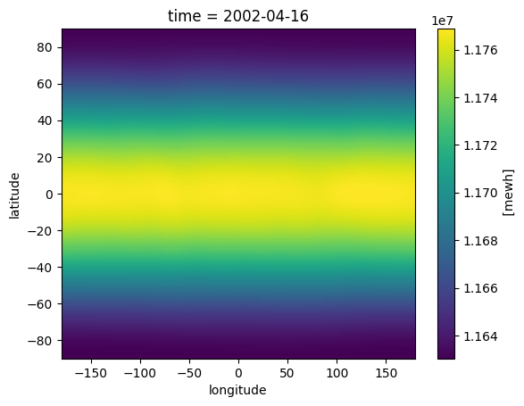
The grid output is a xr.DataArray depending on longitude, latitude (and time if the dimension exist). It can be used as a normal DataArray.
The constant Earth gravity field is dominated by \(C_{2,0}\) coefficient so the dominant variations at one date correspond to Earth oblateness.
[55]:
grid.isel(time=0).plot()
[55]:
<matplotlib.collections.QuadMesh at 0x71d50c1d2790>
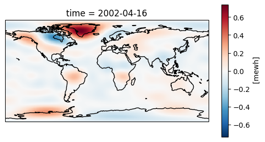
Access residuals and geographic plot
To go futher than an image of the Earth oblatness (\(C_{2,0}\)), we can access the residual of the constant gravity field.
To study time-variable gravity field we need to remove a mean field that gives us access to the residuals values.
It can be done by removing the mean of each Stokes coefficient, or the mean of each grid point, or by substracting an a priori field (e.g. GGM05C for CSR product).
You can also see an example of how to plot geographical maps with matplotlib / xarray.
[56]:
# create grid with residual values
grid_residual = (ds - ds.mean(dim='time')).isel(time=0).lnharmo.to_grid()
You can then visualise the result
[57]:
fig, axis = plt.subplots(1, 1, subplot_kw=dict(projection=ccrs.PlateCarree()))
grid_residual.plot(transform=ccrs.PlateCarree(), cbar_kwargs={'shrink': 0.7})
axis.coastlines()
[57]:
<cartopy.mpl.feature_artist.FeatureArtist at 0x71d50c2678d0>
Going back to Spherical Harmonics
From the spatial values in a DataArray, we can estimate the Stokes coefficients back with da.lnharmo.to_sh()
This writing is equivalent to grid_to_sh(da) (located in lenapy.utils.harmo) so to see the argument that might be used look at the documentation of this function.
You can change the degree \(l\) and order \(m\) that will be estimated and use an ellispoidal Earth. Using kwargs, you can also pass parameters to l_factor_conv** to change the used constants in the unit conversion.
[58]:
grid_residual.lnharmo.to_sh(lmax=60)
[58]:
<xarray.Dataset> Size: 61kB
Dimensions:  (l: 61, m: 61)
Coordinates:
  * l        (l) int64 488B 0 1 2 3 4 5 6 7 8 9 ... 52 53 54 55 56 57 58 59 60
  * m        (m) int64 488B 0 1 2 3 4 5 6 7 8 9 ... 52 53 54 55 56 57 58 59 60
    time     datetime64[ns] 8B 2002-04-16
Data variables:
    clm      (l, m) float64 30kB -4.21e-14 0.0 0.0 ... 8.301e-28 -3.514e-28
    slm      (l, m) float64 30kB 0.0 0.0 0.0 ... -2.675e-27 4.305e-27 1.3e-27
Attributes:
    gm_earth:    398600441500000.0
    a_earth:     6378137.0
    max_degree:  60
norm: 4piManipulating Spherical harmonics datasets
Operation of spherical harmonics dataset
You may have seen that I can apply operation like power (2) over ds.lnharmo object. In fact several methods have been overwriten to be applied only over ds.clm** and ds.slm variables in the dataset.
By this way you can add, subtract, multiply dataset with spherical harmonics variables by applying the operation onto ds.lnharmo object.
Note that you can not apply the divide operation (however, you can multiply by \(\frac{1}{x}\)).
[59]:
ds_sum = ds.isel(time=slice(0)).lnharmo + ds.isel(time=slice(1))

ds_mean = (ds.isel(time=slice(0)).lnharmo + ds.isel(time=slice(1))).lnharmo * 0.5
Plot based on spherical harmonics
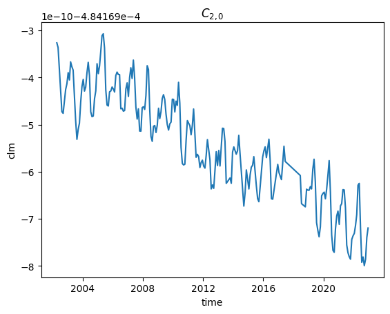
Time-serie plot
You can just the time-series corresponding to one coefficient with ds.sel(l=l, m=m).plot()
If you give argument to the .plot() function they are interpreted as plot argument like ‘label’ or ‘color’.
After the plot, you can modify the matplotlib figure as usual.
[60]:
# time series of one coefficient
ds.isel(l=2, m=0).clm.plot()
plt.title("$C_{2,0}$")
[60]:
Text(0.5, 1.0, '$C_{2,0}$')
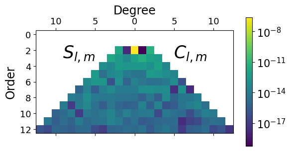
Triangular plot
With a spherical harmonics dataset, we might try to look at it in terms of SH coefficients amplitude with the function ds.lnharmo.plot_hs() that call the function located in lenapy.plots.plotting.
You first need to create a dataset without extra dimension (reduce the time with a .sel(time=…) or a .mean(‘time’) or other). Then you can plot the dataset.
[61]:
import matplotlib.ticker as ticker

# reduce the dataset to one date
ds_square = ds.isel(time=0).lnharmo ** 2

# triangular plot
ax = ds_square.lnharmo.plot_hs(norm='log', lmax=12)
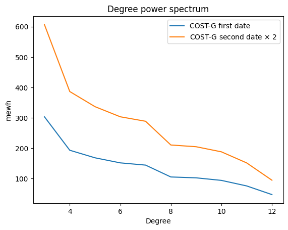
HS power plot
You can plot the degree power for a certain date with the function plot_power_hs() located in lenapy.plots.plotting.
You first need to create a dataset without extra dimension (reduce the time with a .sel(time=…) or other). Then you can plot the dataset.
[62]:
from lenapy.plots.plotting import plot_power

# plot the degree power
plot_power(ds.isel(time=0), lmin=3, label='COST-G first date')
plot_power(ds.isel(time=1).lnharmo*2, lmin=3, label=r'COST-G second date $\times$ 2')
plt.legend()
plt.title("Degree power spectrum")
[62]:
Text(0.5, 1.0, 'Degree power spectrum')
Writing .gfc file
You can write a .gfc file with ds.lnharmo.to_gfc(). The function dataset_to_gfc located in lenapy.writers.gravi_writer allows to write .gfc ascii file from a spherical harmonics dataset.
The writer will inspect ds.attrs to create the header of the gfc file. If values are not contained in ds.attrs or in the function parameters, default values are used.
First, you need to create a dataset without extra dimensions by reducing the ‘time’ dimension using methods like .sel(time=…) or .mean(‘time’).
[15]:
example_path = 'tmp/test.gfc'

# Write the spherical harmonics data of the first time slice to a .gfc file
ds.isel(time=0).lnharmo.to_gfc(example_path)