Climatology
Overview
The climato method from the lntime module enables regression of a signal from a dataset:
on annual or semi-annual cycles
on polynomials of any order
on any user-defined function
It returns an instance of the Coeffs_climato class.
The time sampling can be arbitrary.
Basically, the climato method solves a least squares problem Y = A.X, where Y is a time-dependent signal and X is a matrix of defined temporal functions (annual cycle, mean, trend, acceleration, arbitrary functions, etc.). A thus contains the coefficients to apply to each of these temporal functions to minimize the residuals Y - A.X.
Input dataset format
One dimension must correspond to time. The time variable does not necessarily need to be a coordinate; it can be a variable in the dataset.
There can be any number of dimensions independent of time (latitude, longitude, depth, models, etc.).
Coeffs_climato Class
Initialisation
clim = Coeffs_climato(ds, dim='time', var=None, Nmin=6, cycle=True, order=1)
ds: dataset or dataarray containing the data
dim: name of the dimension over which to perform the regressions
var: name of the variable or coordinate containing time information. If None,
var = dimNmin: minimum number of valid data points required to compute the coefficients. This number is added to the number of regression functions. For example, if
Nmin=0and you’re computing annual and semi-annual cycles, trend, and mean, you need at least 6 valid points; otherwise, the coefficients will be set to NaN.cycle: use annual and semi-annual cycle functions by default
order: polynomial order for regression. If
order = -1, no polynomial regression is applied.
Adding custom functions:
clim.add_coeffs(coefficients, func, *var, ref=None, scale=pd.to_timedelta("1D").asm8, **kwargs)
coefficients: names of the coefficients corresponding to the output of the
funcfunctionfunc: function that takes a time series as input and returns a dataarray
var: variables passed as parameters to the
funcref: temporal origin used in computing the function
scale: time scaling used in computing the function
kwargs: additional parameters passed to the function
The computed function is actually evaluated as: func((x - ref) / scale)
Coefficient computation:
coeffs = clim.solve(measure=None, chunk=None, weight=None, t_min=None, t_max=None)
measure: name of the variable in the input dataset
dsfor which to compute the climatology. If the input is a dataArray, leave this blank.chunk: enables parallel processing for large datasets with multiple dimensions
weight: weighting matrix for the least squares computation. If
None, all measurements are equally weightedt_min, t_max: start and end times for the climatology calculation. If
None, no time limit is applied.
This method returns an instance of the Signal_climato class.
Signal_climato Class
This class is used to work with climatological coefficients. It is returned by the solve method from the Coeffs_climato class, but can also be constructed from previously saved coefficients. In that case, it must be properly initialized with all the parameters of the functions used to perform the regression.
Initialization
signal = Signal_climato(coeffs, dim='time', var=None, cycle=True, order=1, ref=None, ds=None, measure=None)
coeffs: coefficients computed by the Coeffs_climato class
dim: name of the dimension over which to perform the regressions
var: name of the variable or coordinate containing time information. If None,
var = dimcycle: use of annual and semi-annual cycle functions by default
order: polynomial order for regression. If
order = -1, no polynomial regressionref: default reference for built-in functions (annual cycle and polynomial)
ds: dataset or dataarray used for coefficient computation (optional; only used for residual or interpolation calculations)
measure: if
dsis defined and is a dataset, name of the variable containing the measurements used to compute the coefficients
Adding custom functions:
Outputs
signal.climatology(coefficients=None, x=None) :
Regressed climatological function
coefficients: names of coefficients to include in the output time series. If
None, all coefficients are usedx: time points for computation. If
None, time values from the input dataset are used (x = ds.var)
signal.residuals(coefficients=None)
Residuals between measurements and the regressed climatological function
coefficients: names of coefficients to consider for residuals calculation. If
None, all coefficients are used
signal.signal(x=None, coefficients=None, method='linear')
Signal combining interpolated residuals and the regressed climatological function. If residuals contain NaNs, they are interpolated using the chosen method
x: time points for computation. If
None, time values from the input dataset are used (x = ds.var)coefficients: names of coefficients to consider. If
None, all are usedmethod: interpolation method for calculation times and NaN values, from
scipy.interp1doptions
[1]:
import lenapy
import xarray as xr
import os.path
import pandas as pd
import numpy as np
import matplotlib.pyplot as plt
from lenapy.constants import *
Example on a Simple Time Series
[2]:
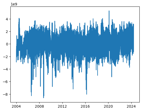
moheacan=xr.open_dataset('../../data/ohc.nc')
moheacan.gohc.plot()
moheacan
[2]:
<xarray.Dataset> Size: 2MB
Dimensions:    (time: 216, latitude: 30, longitude: 30)
Coordinates:
  * time       (time) datetime64[ns] 2kB 2005-01-14T23:46:17.343750 ... 2022-...
  * latitude   (latitude) float64 240B 30.5 31.5 32.5 33.5 ... 57.5 58.5 59.5
  * longitude  (longitude) float64 240B -29.5 -28.5 -27.5 ... -2.5 -1.5 -0.5
Data variables:
    ohc        (time, latitude, longitude) float64 2MB ...
    gohc       (time) float64 2kB ...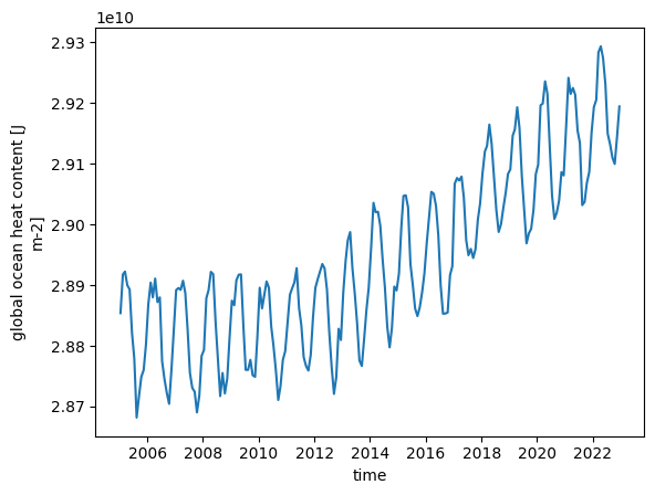
Calling the Climato Class
By default, the regression functions are the annual cycle, the semi-annual cycle, the mean, and the trend.
[3]:
clim=moheacan.gohc.lntime.Coeffs_climato()
clim.coeff_names
[3]:
['cosAnnual',
 'sinAnnual',
 'cosSemiAnnual',
 'sinSemiAnnual',
 'order_0',
 'order_1']
Calculation of Climatology Coefficients on a Dataset Variable
First, the climatology must be calculated by specifying the variable in the input dataset that contains the measurements.
[4]:
clim_gohc=clim.solve()
Calculation of the Corresponding Climate Signal
The climatology method returns the different components of the climate signal. If nothing is specified, the sum of all components is computed. Otherwise, the coefficients parameter should contain a list of the names of the coefficients to return.
The climate signal can be computed at time steps different from those of the original signal. To do this, pass a dataset or data array to the x argument that includes all the variables required to compute the fitted functions. Typically, 'time' is sufficient.
[5]:
moheacan.gohc.plot(label='Measurements')
clim_gohc.climatology().plot(label='All coefficients')
clim_gohc.climatology(coefficients=['order_0','order_1']).plot(label='Mean and trend')
t_new=xr.DataArray(pd.date_range('2000','2024',freq='1MS'),dims=['time'])
clim_gohc.climatology(x=t_new,coefficients=['order_0','order_1','cosAnnual','sinAnnual']).plot(label='Extended period')

plt.legend()
[5]:
<matplotlib.legend.Legend at 0x145f8ec850d0>
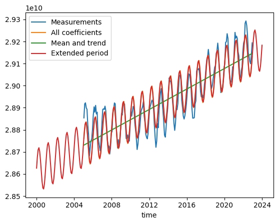
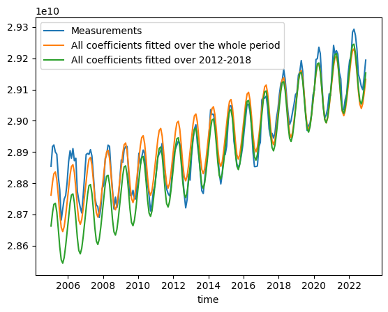
Climatology can be computed over a restricted period by using the t_min and t_max parameters.
[6]:
moheacan.gohc.plot(label='Measurements')
clim.solve('gohc').climatology().plot(label='All coefficients fitted over the whole period')
clim.solve('gohc',t_min='2012',t_max='2018').climatology().plot(label='All coefficients fitted over 2012-2018')

plt.legend()
[6]:
<matplotlib.legend.Legend at 0x145f8ed10150>
## Using custom fit functions
The functions to be fitted are called by applying a reference and scaling to the input data: func((t - tref) / scale)
The default functions for annual and semi-annual cycles, mean, and trend used when instantiating the Climato class apply the first date of the time series as the reference, and use a scaling so that the time unit is one day.
Using one of the two functions instantiated in the
Climatoclass:poly(order, ref, scale): creates a polynomial function of the chosen order, with optional reference and scaling.
cycle(ref): generates annual and semi-annual cycles, with optional reference.
Using the
add_coeffsmethod to define a custom function:First, define a function of one or more variables that returns a DataArray with two dimensions:
One dimension matching that of the dataset used for climatology computation (most commonly
'time'),Another called
'coeffs', allowing multiple functions to be returned in a single call.
The function should have the form func(p1, p2, p3, …), and will be called as func((p1 - ref) / scale, p2, p3, …)
Assign this function to the
Climatoinstance using the add_coeffs(coefficients, func, args, ref, scale)* method:coefficients: list of component names for the function to be fitted (sinAnnual, trend, acc, … of your choice).
func: the previously defined function.
args: one or more names of the dataset variables that are function parameters (usually time, but can be any variable).
ref and scale: reference and scaling, applied only to the first argument of the function. By default, ref is the minimum value of the variable, and scale is
pd.to_timedelta("1D").asm8(i.e., 1 day).
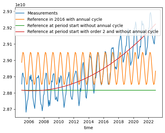
[10]:
moheacan.gohc.plot(label='Measurements')

clim=moheacan.lntime.Coeffs_climato(cycle=True,order=2,ref=pd.to_datetime('2016').asm8)
clim_gohc = clim.solve('gohc')
clim_gohc.climatology(coefficients=['order_0','cosAnnual','sinAnnual']).plot(label='Reference in 2016 with annual cycle')

clim=moheacan.lntime.Coeffs_climato(cycle=False,order=2)
clim_gohc=clim.solve('gohc')
clim_gohc.climatology(coefficients=['order_0']).plot(label='Reference at period start without annual cycle')
clim_gohc.climatology(coefficients=['order_0','order_1','order_2']).plot(label='Reference at period start with order 2 and without annual cycle')

plt.legend()
[10]:
<matplotlib.legend.Legend at 0x145f86338150>
[13]:
# Example of the Default Implemented Functions:
omega=2*np.pi/LNPY_DAYS_YEAR
def annual(x):
return xr.concat((np.cos(omega*x),np.sin(omega*x)),dim="coeffs")
def semiannual(x):
return xr.concat((np.cos(2*omega*x),np.sin(2*omega*x)),dim="coeffs")
def pol(x,order=1):
return x**xr.DataArray(np.arange(order+1),dims='coeffs')
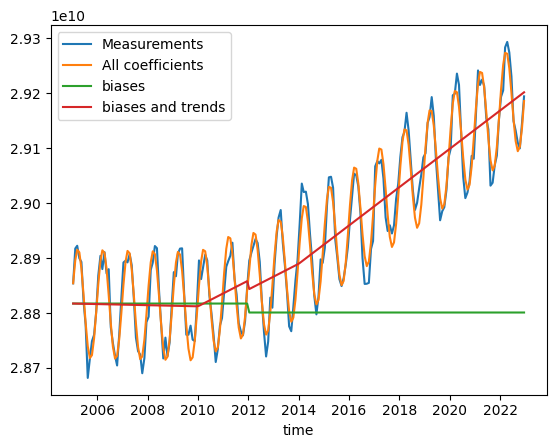
# Example of a Function to Add a Second Trend and a Bias Starting from a Given Date:
def trend(x):
return xr.where(x<0,0,x)
def bias(x):
return xr.where(x<0,0,1.)
# Adding Functions to Fit to the Climato Instance
clim=moheacan.lntime.Coeffs_climato(cycle=False,order=1)
# Annual cycle
clim.add_coeffs(['cosAnnual','sinAnnual'],annual,'time')
# Second biais since 2012
clim.add_coeffs('bias2',bias,'time',ref=pd.to_datetime('2012').asm8)
# Second trend since 2010
clim.add_coeffs('trend2',trend,'time',ref=pd.to_datetime('2010').asm8)
# Third Trend Starting from 2014 (using the same function)
clim.add_coeffs('trend3',trend,'time',ref=pd.to_datetime('2014').asm8)
clim_gohc = clim.solve('gohc')
moheacan.gohc.plot(label='Measurements')
clim_gohc.climatology().plot(label='All coefficients')
clim_gohc.climatology(['order_0','bias2']).plot(label='biases')
clim_gohc.climatology(['order_0','bias2','order_1','trend2','trend3']).plot(label='biases and trends')
plt.legend()
[13]:
<matplotlib.legend.Legend at 0x145f85df0090>
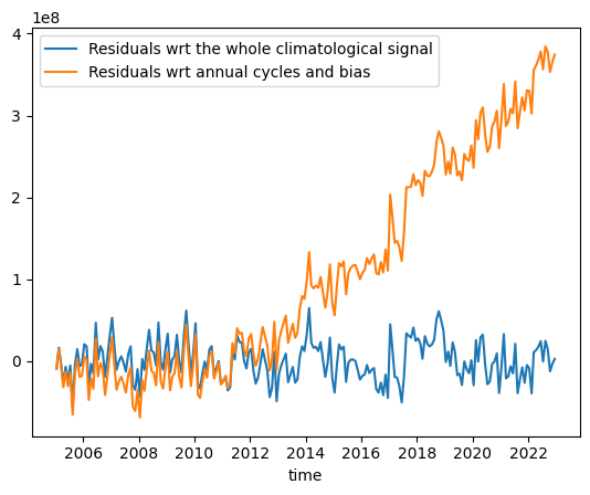
Calculation of Residuals
The residuals method returns the residuals of the input signal relative to the climate signal. You can choose which coefficients to include in the climate signal.
[14]:
clim=moheacan.lntime.Coeffs_climato(order=3)
clim_gohc = clim.solve('gohc')
clim_gohc.residuals().plot(label='Residuals wrt the whole climatological signal')
clim_gohc.residuals(coefficients=['sinAnnual','cosAnnual','sinSemiAnnual','cosSemiAnnual','order_0']).plot(label='Residuals wrt annual cycles and bias')
plt.legend()
[14]:
<matplotlib.legend.Legend at 0x145f84f66590>
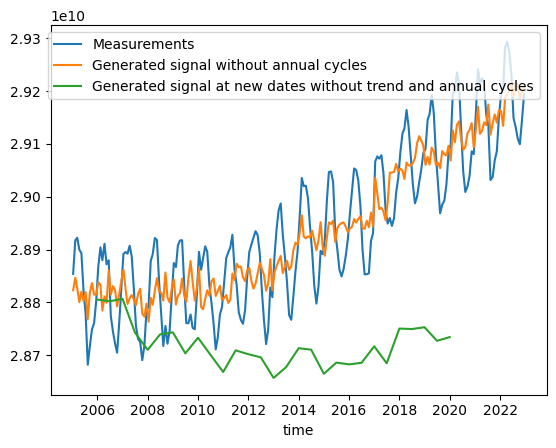
Generation of a Signal and Interpolation
The signal method allows generating the original signal by:
including the coefficients of the desired climate signal components,
interpolating the NaN values in the residuals of the original signal using an interpolation method available in
scipy.interp1d,interpolating at dates different from those of the original signal (no extrapolation possible).
(Note: This last interpolation feature does not work if the climate functions take arguments other than time as input, since that would require multi-dimensional interpolation, which is beyond the scope of this class.)
[15]:
moheacan.gohc.plot(label='Measurements')

clim=moheacan.lntime.Coeffs_climato(order=1)
clim_gohc = clim.solve('gohc')
clim_gohc.signal(coefficients=['order_0','order_1']).plot(label='Generated signal without annual cycles')
t_new=xr.DataArray(pd.date_range('2006','2020',freq='6MS'),dims='time')
clim_gohc.signal(x=t_new,coefficients=['order_0']).plot(label='Generated signal at new dates without trend and annual cycles')
plt.legend()
[15]:
<matplotlib.legend.Legend at 0x145f84fd9f50>
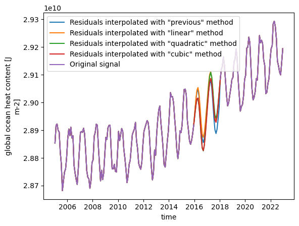
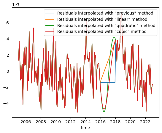
Example of Interpolation by Setting Two Years of Measurements to NaN.
[16]:
trous=moheacan.where((moheacan.time<pd.to_datetime('2016'))|(moheacan.time>pd.to_datetime('2018')))
clim=trous.lntime.Coeffs_climato(order=2)
clim_gohc = clim.solve('gohc')

# Reconstructed Signal with All Climatology Components, Residuals Interpolated Using Various Methods
clim_gohc.signal(method='previous').plot(label='Residuals interpolated with "previous" method')
clim_gohc.signal(method='linear').plot(label='Residuals interpolated with "linear" method')
clim_gohc.signal(method='quadratic').plot(label='Residuals interpolated with "quadratic" method')
clim_gohc.signal(method='cubic').plot(label='Residuals interpolated with "cubic" method')

trous.gohc.plot(label='Original signal')
plt.legend()
[16]:
<matplotlib.legend.Legend at 0x145f84e6a810>
[17]:
# Residuals Only, Interpolated Using Various Methods

clim_gohc.signal(coefficients=[],method='previous').plot(label='Residuals interpolated with "previous" method')
clim_gohc.signal(coefficients=[],method='linear').plot(label='Residuals interpolated with "linear" method')
clim_gohc.signal(coefficients=[],method='quadratic').plot(label='Residuals interpolated with "quadratic" method')
clim_gohc.signal(coefficients=[],method='cubic').plot(label='Residuals interpolated with "cubic" method')

plt.legend()
[17]:
<matplotlib.legend.Legend at 0x145f84f66450>
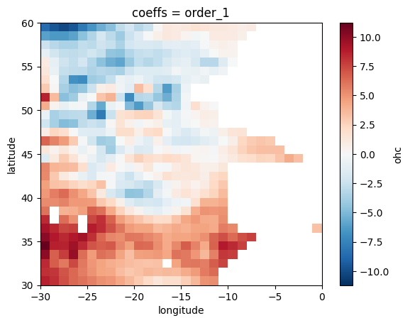
Climatology on a Grid
[20]:
clim=moheacan.lntime.Coeffs_climato(order=1)
clim_ohc = clim.solve('ohc')
clim_ohc.result.sel(coeffs='order_1').plot()
[20]:
<matplotlib.collections.QuadMesh at 0x145f84c87fd0>
Climatology on Irregular Points
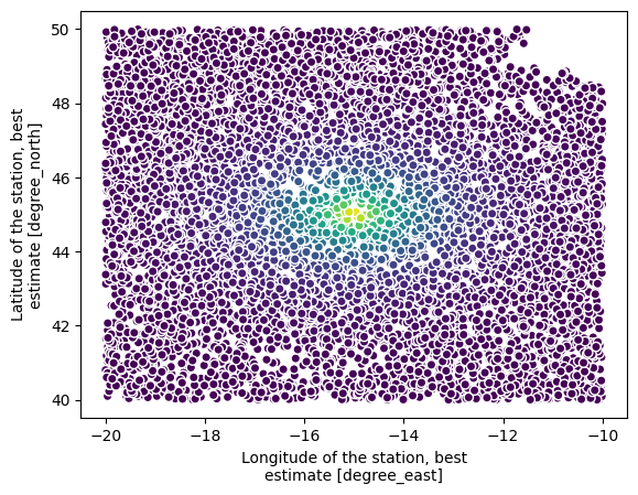
[21]:
argo=xr.open_dataset('../../data/argo.nc')
argo.plot.scatter(x='longitude',y='latitude',c=argo.ohc)
argo
[21]:
<xarray.Dataset> Size: 260kB
Dimensions:    (N_PROF: 8124)
Dimensions without coordinates: N_PROF
Data variables:
    latitude   (N_PROF) float64 65kB ...
    longitude  (N_PROF) float64 65kB ...
    time       (N_PROF) datetime64[ns] 65kB ...
    ohc        (N_PROF) float64 65kB 3.301e+10 3.092e+10 ... 3.439e+10 3.549e+10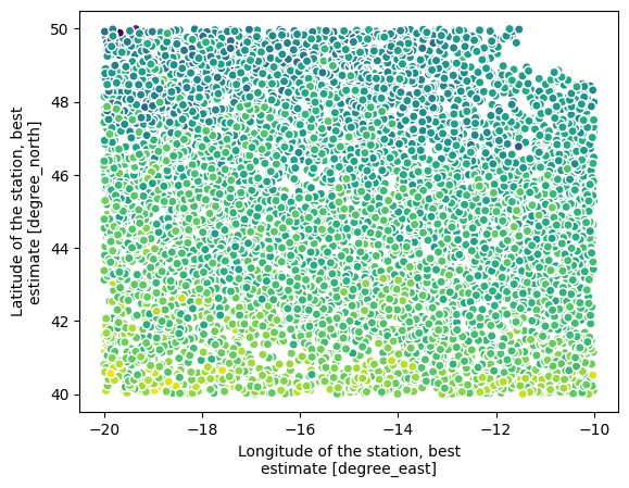
To compute a heat climatology in this area, you need to specify the dimension along which to perform the calculations (N_PROF) and the name of the variable containing the date (time).
[22]:
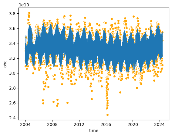
clim=argo.lntime.Coeffs_climato(dim='N_PROF',var='time')
clim_ohc = clim.solve('ohc')
[23]:
plt.plot(argo.time,clim_ohc.climatology())
argo.plot.scatter(x='time',y='ohc',c='orange')
[23]:
<matplotlib.collections.PathCollection at 0x145f84b18f50>
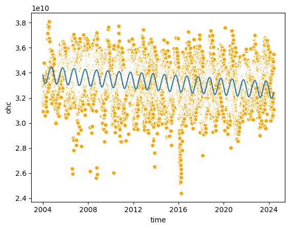
This climatology does not account for the latitude gradient; the measurements are very scattered and the residuals are large.
[24]:
plt.plot(argo.time,clim_ohc.residuals())
[24]:
[<matplotlib.lines.Line2D at 0x145f84ba7950>]
A regression can be performed on the deviation in latitude and longitude relative to the center of the area.
[25]:
def f(X):
    return X

clim2=argo.lntime.Coeffs_climato(dim='N_PROF',var='time',order=3)
clim2.add_coeffs('GradLat',f,'latitude',ref=45,scale=1.)
clim2.add_coeffs('GradLon',f,'longitude',ref=-15,scale=1.)
clim_ohc2 = clim2.solve('ohc')

plt.plot(argo.time,clim_ohc2.climatology())
argo.plot.scatter(x='time',y='ohc',c='orange')
[25]:
<matplotlib.collections.PathCollection at 0x145f84b38510>
We can see that the climatology including the positional gradient better reflects reality, and the residuals are smaller.
[26]:
plt.plot(argo.time,clim_ohc.residuals(),label='Without position gradient')
plt.plot(argo.time,clim_ohc2.residuals(),label='With position gradient')
plt.legend()
[26]:
<matplotlib.legend.Legend at 0x145f84ba1e90>
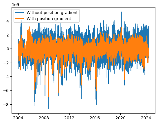
The residuals are much closer to white noise.
[27]:
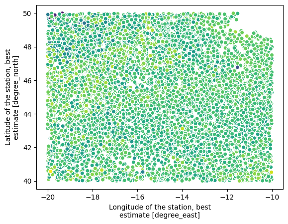
argo.plot.scatter(x='longitude',y='latitude',c=clim_ohc2.residuals())
[27]:
<matplotlib.collections.PathCollection at 0x145f84a35510>
It is also possible, when calculating the climatology at a point, to add weights based on the distance from the measurement to that point.
[28]:
# Calculation of the Weighting Function and Plotting the Weights for All Measurement Points
sig_dist=100000.
centre=xr.DataArray(data=0,dims=['latitude','longitude'],coords=dict(latitude=[45],longitude=[-15]))
dist=centre.lngeo.distance(argo).squeeze().drop_vars(['latitude','longitude'])
poids=np.exp(-(dist/sig_dist))
argo['poids']=poids/poids.sum('N_PROF')
arg=argo.sortby(poids)
argo.plot.scatter(x='longitude',y='latitude',c=poids)
[28]:
<matplotlib.collections.PathCollection at 0x145f849c7690>
[29]:
clim_ohc2 = clim2.solve('ohc',weight=poids)

plt.scatter(x=argo.time,y=argo.ohc,c=argo.poids,s=5,vmax=0.0005)

t=xr.Dataset(coords=dict(time=pd.date_range('2004','2024',freq='1MS')))
z=xr.zeros_like(t.time.astype(float))
t_new=xr.Dataset(dict(latitude=z+45,longitude=z-15))
clim_ohc2.climatology(x=t_new,coefficients=['order_0','order_1','order_2','order_3','cosAnnual','sinAnnual']).plot(lw=2,c='r')
plt.ylim([3e10,3.7e10])
t_new
[29]:
<xarray.Dataset> Size: 6kB
Dimensions:    (time: 241)
Coordinates:
  * time       (time) datetime64[ns] 2kB 2004-01-01 2004-02-01 ... 2024-01-01
Data variables:
    latitude   (time) float64 2kB 45.0 45.0 45.0 45.0 ... 45.0 45.0 45.0 45.0
    longitude  (time) float64 2kB -15.0 -15.0 -15.0 -15.0 ... -15.0 -15.0 -15.0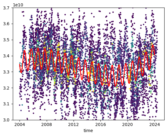
[30]:
clim_ohc2.result.to_netcdf('climato_sparse.nc')
Using Climatology Coefficients Independently of the Original Signal
For example, if the “result” attribute of the Climato instance has been saved, you might want to recreate a signal after reloading these coefficients. To do this, you need to know all the parameters used to generate this climatology:
the names of the coefficients
the names of the associated functions
the names of the variables for the functions
the reference and scaling
any additional parameters to pass to the function (e.g., the order for the polynomial to regress)
Climato class.Climato class, the annual and semi-annual cycles, as well as the mean and trend, are added with a default reference which will be the minimum date of the time series on which the signal is calculated. If you do not want these default functions, specify cycle=False and/or order=-1 when calling the class.Then call climatology exactly as with the Climato instance, except that it is mandatory to specify the vector on which to calculate the signal. This vector is a dataset or data array containing the variables necessary for executing the climatology functions (usually time).
It is not mandatory to assign a function to all present coefficients; in that case, only the coefficients for which a function has been defined will be calculated.
[31]:
clim_saved=xr.open_dataset('climato_sparse.nc')
clim_saved
[31]:
<xarray.Dataset> Size: 600B
Dimensions:  (coeffs: 10)
Coordinates:
  * coeffs   (coeffs) <U13 520B 'cosAnnual' 'sinAnnual' ... 'GradLat' 'GradLon'
Data variables:
ohc (coeffs) float64 80B ...[32]:
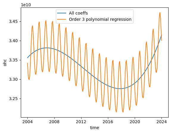
from lenapy.utils.climato import Signal_climato
# An instance is created with the annual cycle functions and without polynomial regression. (var and cycle are unnecessary as they are the default values)
generate = Signal_climato(clim_saved, var='time', cycle=True, order=-1)
# For educational purposes, to add a polynomial function, use the add_coeffs method specifying:
#  - the names of the coefficients concerned in "clim_saved"
#  - the name of the function to apply (pol)
#  - the name of the variable on which to apply the function
#  - the reference (None: this will be the minimum value of the variable on which to calculate the signal) (not needed here as it is the default if absent)
#  - the scaling (not needed here as it is the default if absent)
#  * additional parameters for the function (the polynomial order)
generate.add_coeffs(['order_%i'%i for i in np.arange(4)],pol,'time', ref=None, scale=pd.to_timedelta("1D").asm8, order=3)

# No function has been defined for gradLat and gradLon; these coefficients will not be used in the output signal.
[33]:
generate.climatology(x=t_new,coefficients=['order_0','order_1','order_2','order_3']).ohc.plot(label='All coeffs')
generate.climatology(x=t_new).ohc.plot(label='Order 3 polynomial regression')
plt.legend()
[33]:
<matplotlib.legend.Legend at 0x145f7fc50050>
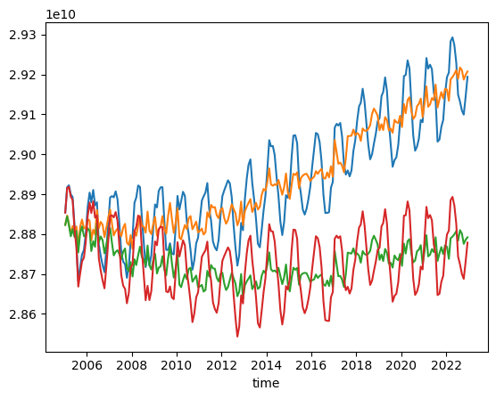
Ascending Compatibility
[34]:
moheacan.gohc.plot(label='Measurements')
moheacan.gohc.lntime.climato().plot()
moheacan.gohc.lntime.climato(trend=False).plot()
moheacan.gohc.lntime.climato(trend=False,cycle=True).plot()
[34]:
[<matplotlib.lines.Line2D at 0x145f7fcf2350>]
[ ]: